Project Part 1

Preparing the Gender Gap in Median Earnings Data for Plotting

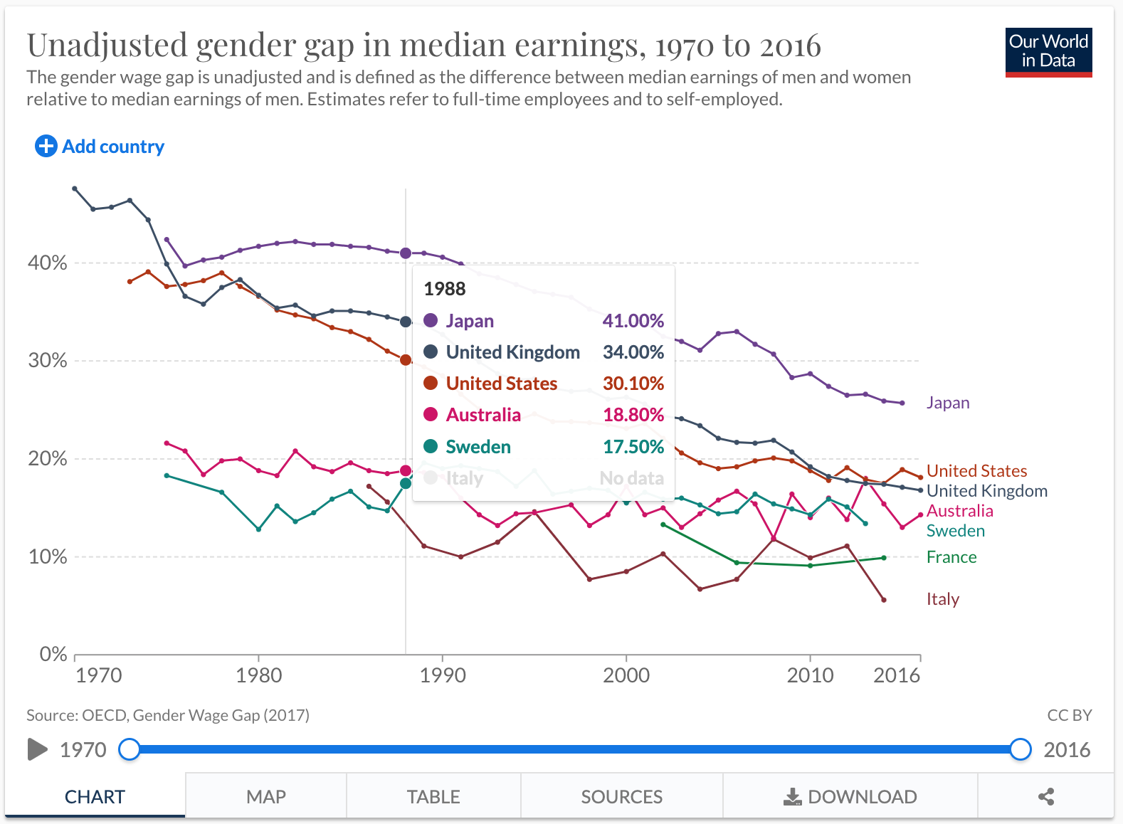
1. I downloaded gender gap in median earnings data from Our World in Data. I selected this data because I’m interested in which country is combating the gender wage gap the best from 1970 to 2016.

2. This is the link to the data.

3. The following code chunk loads the package I will use to read in and prepare the data for analysis

library(tidyverse)

4. Read the data in

gender_wage_gap_oecd <- read_csv(here::here("_posts/2022-05-07-project-part-1/gender-wage-gap-oecd.csv"))

5. Use glimpse to see the names and types of the columns

glimpse(gender_wage_gap_oecd)

Rows: 636
Columns: 4
$ Entity                        <chr> "Australia", "Australia", "Aus…
$ Code                          <chr> "AUS", "AUS", "AUS", "AUS", "A…
$ Year                          <dbl> 1975, 1976, 1977, 1978, 1979, …
$ `Gender wage gap (OECD 2017)` <dbl> 21.6, 20.8, 18.4, 19.8, 20.0, …

#view(gender_wage_gap_oecd)

6. Use output from glimpse (and View) to prepare the data for analysis

• Create the object country that is list of countries I want to extract from the dataset
• Change the name of 1st column to Country and the 4th column to WageGap
• Use filter to extract the rows that I want to keep: Year >= 1970 and country in countries
• Select the columns to keep: Country, Year, WageGap
• Assign the output to country_wageGap
• Display the first 10 rows of country_wageGap

countries  <- c("Japan",
               "United States",
               "United Kingdom",
               "Australia",
               "Sweden",
               "France",
               "Italy")

country_wageGap <- gender_wage_gap_oecd  %>% 
  rename(country = 1, WageGap = 4)  %>% 
  filter(Year >= 1970, country %in%  countries)  %>% 
  select(country, Year, WageGap) 

country_wageGap

# A tibble: 228 × 3
   country    Year WageGap
   <chr>     <dbl>   <dbl>
 1 Australia  1975    21.6
 2 Australia  1976    20.8
 3 Australia  1977    18.4
 4 Australia  1978    19.8
 5 Australia  1979    20  
 6 Australia  1980    18.8
 7 Australia  1981    18.3
 8 Australia  1982    20.8
 9 Australia  1983    19.2
10 Australia  1984    18.7
# … with 218 more rows

Add a picture.

See how to change the width in the R Markdown Cookbook

Countries Wage Gaps

Write the data to file in the project directory

write_csv(country_wageGap, file="country_wageGap.csv")